Boosting 이란?

• 여러 개의 약한 Decision Tree를 조합해서 사용하는 Ensemble 기법 중 하나이다.
  • 즉, 약한 예측 모형들의 학습 에러에 가중치를 두고, 순차적으로 다음 학습 모델에 반영하여
  • 강한 예측모형을 만드는 것이다.

XGBoost 란?

• XGBoost는 Extreme Gradient Boosting의 약자이다.
• Boosting 기법을 이용하여 구현한 알고리즘은 Gradient Boost 가 대표적인데
• 이 알고리즘을 병렬 학습이 지원되도록 구현한 라이브러리가 XGBoost 이다.
• Regression, Classification 문제를 모두 지원하며, 성능과 자원 효율이 좋아서, 인기 있게 사용되는 알고리즘이다.

XGBoost의 장점

• GBM 대비 빠른 수행시간
  • 병렬 처리로 학습, 분류 속도가 빠르다.
• 과적합 규제(Regularization)
  • 표준 GBM 경우 과적합 규제기능이 없으나, XGBoost는 자체에 과적합 규제 기능으로 강한 내구성 지닌다.
• 분류와 회귀영역에서 뛰어난 예측 성능 발휘
  • 즉, CART(Classification and regression tree) 앙상블 모델을 사용
• Early Stopping(조기 종료) 기능이 있음
• 다양한 옵션을 제공하며 Customizing이 용이하다.

하이퍼파라미터 튜닝

• reference

  • https://xgboost.readthedocs.io/en/latest/python/python_api.html

• XGBRegressor 하이퍼파라미터 예

    XGBRegressor(base_score=0.5, booster='gbtree', colsample_bylevel=1,
                   colsample_bynode=1, colsample_bytree=1, gamma=0, gpu_id=-1,
                   importance_type='gain', interaction_constraints='',
                   learning_rate=0.1, max_delta_step=0, max_depth=5,
                   min_child_weight=1, missing=nan, monotone_constraints='()',
                   n_estimators=100, n_jobs=0, num_parallel_tree=1, random_state=0,
                   reg_alpha=0, reg_lambda=1, scale_pos_weight=1, subsample=1,
                   tree_method='exact', validate_parameters=1, verbosity=None)
  

• XGBoost는 다수의 하이퍼파라미터가 존재하며, 다음 세가지 범주로 나뉜다.

  • 일반 파라미터
    • 부스팅을 수행할 때 트리를 사용할지, 선형 모델을 사용할지 등을 고른다.
  • 부스터 파라미터
    • 선택한 부스터에 따라서 적용할 수 있는 파라미터 종류가 다르다.
  • 학습 과정 파라미터
    • 학습 시나리오를 결정한다.

• 일반 파라미터

  • booster [기본값 = gbtree]
    • 어떤 부스터 구조를 쓸지 결정한다.
    • 의사결정기반모형(gbtree), 선형모형(gblinear), dart가 있다.
  • n_jobs
    • XGBoost를 실행하는 데 사용되는 병렬 스레드 수
  • verbosity [기본값 = 1]
    • 유효한 값은 0 (무음), 1 (경고), 2 (정보), 3 (디버그)

• 부스터 파라미터

  • gbtree Booster의 파라미터
    • learning_rate [ 기본값 : 0.3 ]
      • learning rate이다.
      • learning rate가 높을수록 과적합 하기 쉽다.
    • n_estimators [ 기본값 : 100 ]
      • 생성할 weak learner의 수
      • learning_rate가 낮을 땐, n_estimators를 높여야 과적합이 방지된다.
    • max_depth [ 기본값 : 6 ]
      • 트리의 maximum depth이다.
      • 적절한 값이 제시되어야 하고 보통 3-10 사이 값이 적용된다.
      • max_depth가 높을수록 모델의 복잡도가 커져 과적합 하기 쉽다.
    • min_child_weight [ 기본값 : 1 ]
      • 관측치에 대한 가중치 합의 최소를 말한다.
      • 값이 높을수록 과적합이 방지된다.
    • gamma [ 기본값 : 0 ]
      • 리프노드의 추가분할을 결정할 최소손실 감소값이다.
      • 해당값보다 손실이 크게 감소할 때 분리한다.
      • 값이 높을수록 과적합이 방지된다.
    • subsample [ 기본값 : 1 ]
      • weak learner가 학습에 사용하는 데이터 샘플링 비율이다.
      • 보통 0.5 ~ 1 사용된다.
      • 값이 낮을수록 과적합이 방지된다.
    • colsample_bytree [ 기본값 : 1 ]
      • 각 tree 별 사용된 feature의 퍼센테이지이다.
      • 보통 0.5 ~ 1 사용된다.
      • 값이 낮을수록 과적합이 방지된다.
    • lambda [기본값 = 1, 별칭 : reg_lambda]
      • 가중치에 대한 L2 Regularization 적용 값
      • 피처 개수가 많을 때 적용을 검토
      • 이 값이 클수록 과적합 감소 효과
    • alpha [기본값 = 0, 별칭 : reg_alpha]
      • 가중치에 대한 L1 Regularization 적용 값
      • 피처 개수가 많을 때 적용을 검토
      • 이 값이 클수록 과적합 감소 효과

• 학습 과정 파라미터

  • objective [ 기본값 : reg = squarederror ]
    • reg : squarederror
      • 제곱 손실이 있는 회귀
    • binary : logistic (binary-logistic classification)
      • 이항 분류 문제 로지스틱 회귀 모형으로 반환값이 클래스가 아니라 예측 확률
    • multi : softmax
      • 다항 분류 문제의 경우 소프트맥스(Softmax)를 사용해서 분류하는데 반횐되는 값이 예측확률이 아니라 클래스임. 또한 num_class도 지정해야함.
    • multi : softprob
      • 각 클래스 범주에 속하는 예측확률을 반환함.
    • count : poisson (count data poison regression) 등 다양하다.
  • eval_metric
    • 모델의 평가 함수를 조정하는 함수다.
    • 설정한 objective 별로 기본설정값이 지정되어 있다.
    • rmse: root mean square error
    • mae: mean absolute error
    • logloss: negative log-likelihood
    • error: Binary classification error rate (0.5 threshold)
    • merror: Multiclass classification error rate
    • mlogloss: Multiclass logloss
    • auc: Area under the curve
    • map (mean average precision)등, 해당 데이터의 특성에 맞게 평가 함수를 조정한다.
  • seed [ 기본값 : 0 ]
    • 재현가능하도록 난수를 고정시킴.

• 민감하게 조정해야하는 것

  • booster 모양
  • eval_metric(평가함수) / objective(목적함수)
  • eta
  • L1 form (L1 레귤러라이제이션 폼이 L2보다 아웃라이어에 민감하다.)
  • L2 form

• 과적합 방지를 위해 조정해야하는 것

  • learning rate 낮추기 → n_estimators은 높여야함
  • max_depth 낮추기
  • min_child_weight 높이기
  • gamma 높이기
  • subsample, colsample_bytree 낮추기

Sample code 1. XGBClassifier

import xgboost as xgb
import matplotlib.pyplot as plt

# 모델 선언
model = xgb.XGBClassifier() 

# 모델 훈련
model.fit(x,y) 

# 모델 예측
y_pred = model.predict(X_test)

Sample code 2. XGBRegressor

import xgboost as xgb

# 모델 선언
my_model = xgb.XGBRegressor(learning_rate=0.1,max_depth=5,n_estimators=100)

# 모델 훈련
my_model.fit(X_train, y_train, verbose=False)

# 모델 예측
y_pred = my_model.predict(X_test) 

시각화

• XGBoost 모형을 시각화함으로써 개발한 예측모형의 성능에 대해 더 깊은 이해를 가질 수 있다.

• 특히 의사결정나무 시각화를 위해서 graphviz 라이브러리 설치가 필요한데, 경로명 설정문제도 함께 해결하는 방식으로 아래와 같이 pip install, conda install 명령어를 연이어 실행시킨다.

    pip install graphviz
    conda install graphviz
  

• xgb.plot_importance() 메쏘드에 XGBoost 모형객체를 넣어 변수중요도를 파악할 수 있다.

    import xgboost as xgb
    
    xgb.plot_importance(my_model)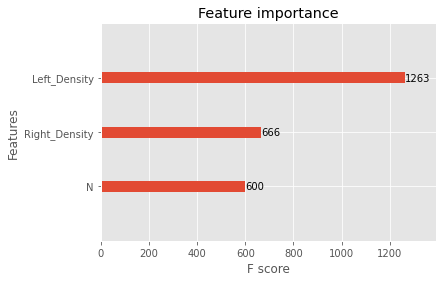
  

  

• xgb.plot_tree() 메쏘드에 XGBoost 모형객체를 넣어 의사결정트리를 시각화할 수 있다.

  • 기본값으로 트리를 저장하면 읽을 수 없을 정도로 낮은 해상도의 이미지가 생성된다.

  • 이미지 크기 또는 해상도를 지정하는 옵션을 다음과 같이 지정해야한다.

      import xgboost as xgb
      import matplotlib.pyplot as plt
        
      # num_trees : 그림을 여러개 그릴시 그림 번호
      # rankdir : 트리의 방향, 디폴트는 위아래 방향
      # rankdir="LR" : 왼쪽에서 오른쪽 방향으로 트리를 보여준다.
      xgb.plot_tree(my_model, num_trees=0, rankdir='LR')
        
      fig = plt.gcf()
      fig.set_size_inches(150, 100)
        
      # 이미지 저장하고 싶다면
      # fig.savefig('tree.png')
        
      plt.show()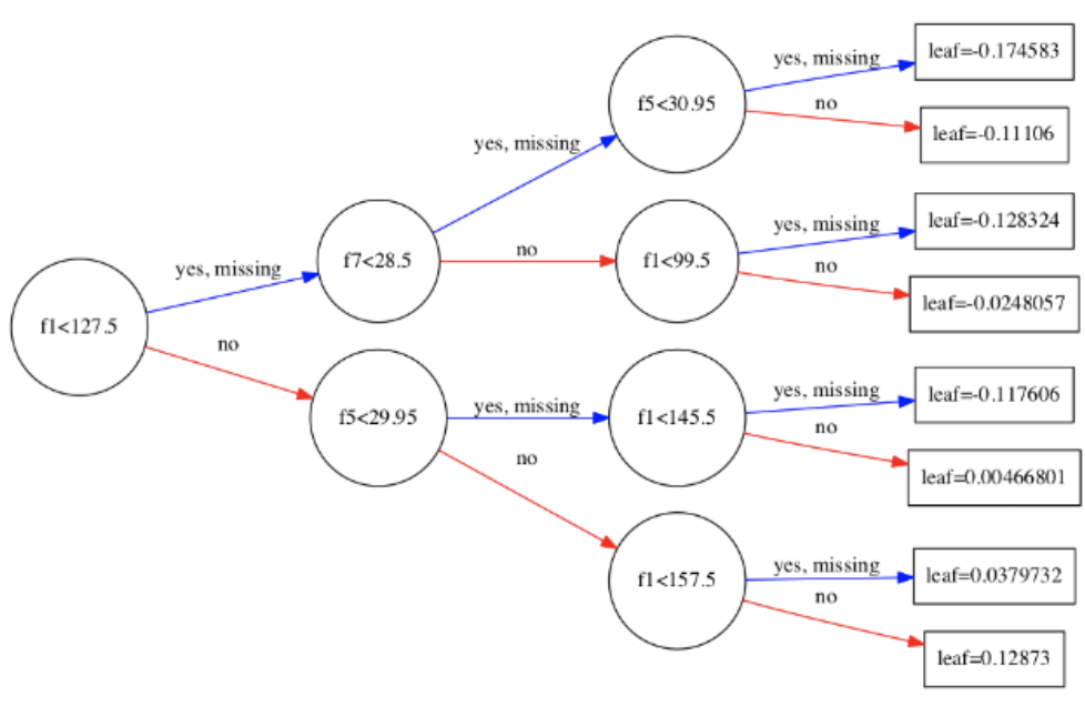
    

    

Source : https://wooono.tistory.com/97